A Review of MoR and TMM Normalization
Set Up
Let y_{i,g} denote the observed count in a sample i \in \mathcal{I} (with n_i = |\mathcal{I}|) for a gene g \in \mathcal{G} (with n_g = |\mathcal{G}|) realized from a particular negative binomial distribution:
\begin{aligned} Y_{i,g} &\sim \text{NegBinom}(\mu_{i,g}, \phi_{g}) \\ \mu_{i,g} &= \eta_{i,g} \cdot \rho_{i} \end{aligned}
Where \eta_{i,g} denotes the true magnitude of expression and \rho_{i} denotes the “size factor” that scales this expression from its ground-truth.
DESeq2’s Median of Ratios
We first focus on a particular gene g and compare the observed count for a sample i to the geometric average of counts across samples to get a ratio R_{i,g}:
R_{i,g} = \frac{ y_{i,g} }{( \prod_{i \in \mathcal{I}} y_{i,g} )^{ \frac{1}{n_i} } }
We then take the median of these ratios to get our size factor estimates!
\hat{s}_{i} = \underset{g \in \mathcal{G}}{\text{median }} R_{i,g}
edgeR’s Trimmed Mean of M Values
We first “normalize” the observed count profile for a sample i by the total number of counts N_i = \sum_{g \in \mathcal{G}} y_{i,g} in order to get proportions:
y'_{i,g} = \frac{y_{i,g}}{N_i}
We next select a reference sample i^{\dagger} \in \mathcal{I} and compute both the ratio of log-transformed proportions and their weights:
\begin{aligned} R_{i,g} &= \frac{\log_2 y'_{i,g}}{\log_2 y'_{i^{\dagger}, g}} \\ w_{i,g} &= \frac{ N_i - y_{i,g} }{ N_i y_{i,g} } + \frac{ N_{i^{\dagger}} - y_{i^{\dagger},g} }{ N_{i^{\dagger}} y_{i^{\dagger},g} } \end{aligned}
We then filter the genes to a subset \mathcal{G}'_i \subset \mathcal{G} by symmetrically “trimming” away the smallest and largest ratios for a sample i to XX% of the original number (defaults to 70%).
We finally compute the “normalization” factor (distinct from a size factor) by taking the weighted average of these ratios and raising it to the second power:
\log_2 \hat{f}_i = \frac{ \sum_{g \in \mathcal{G}'_i} w_{i,g} R_{i,g} }{ \sum_{g \in \mathcal{G}'_i} w_{i,g} }
The size factor is then found by taking the product with the total number of observed counts:
\hat{s}_i = N_i \hat{f}_i
Note: This is referred to as the “effective library size” by the edgeR authors.
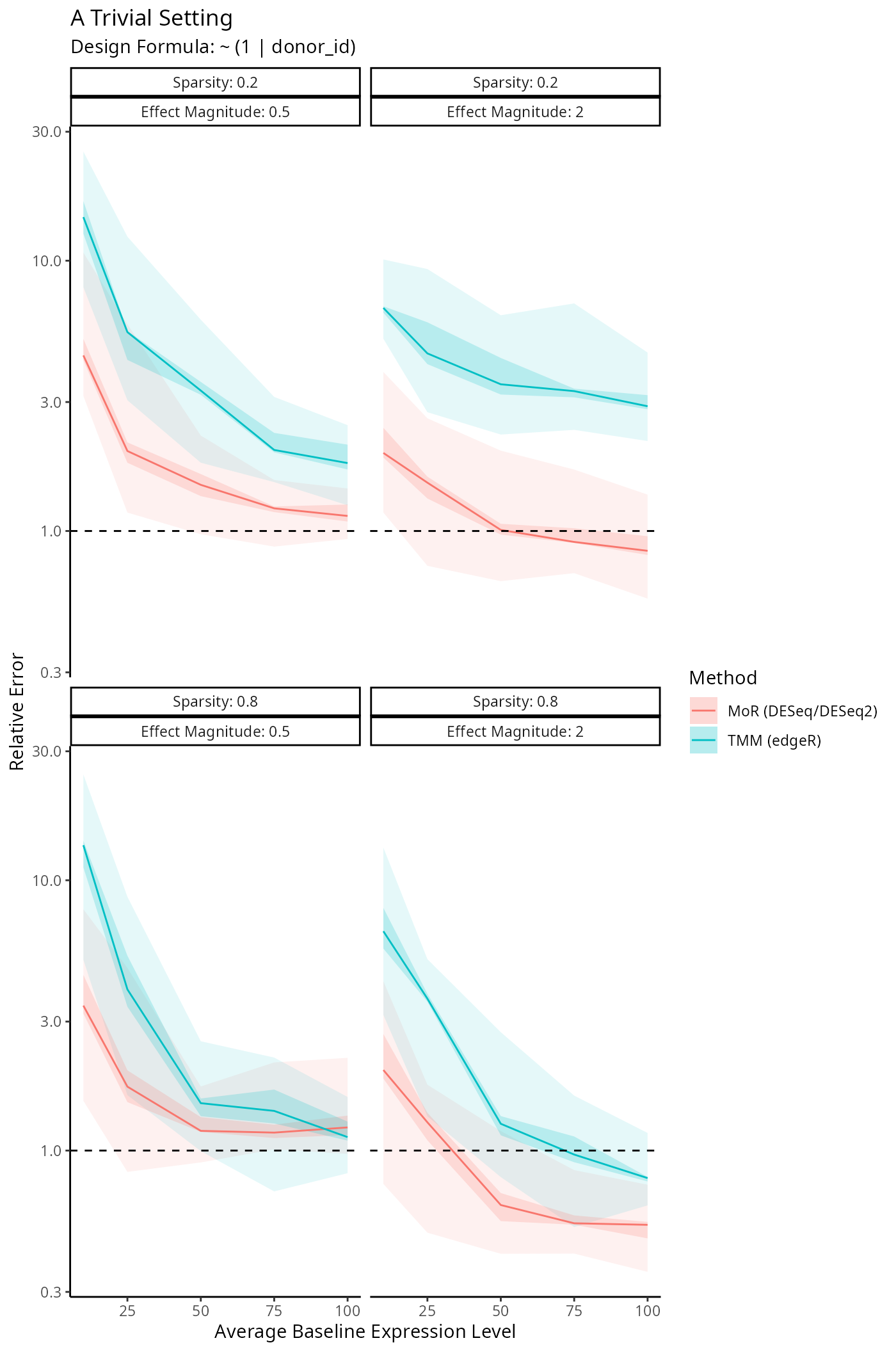
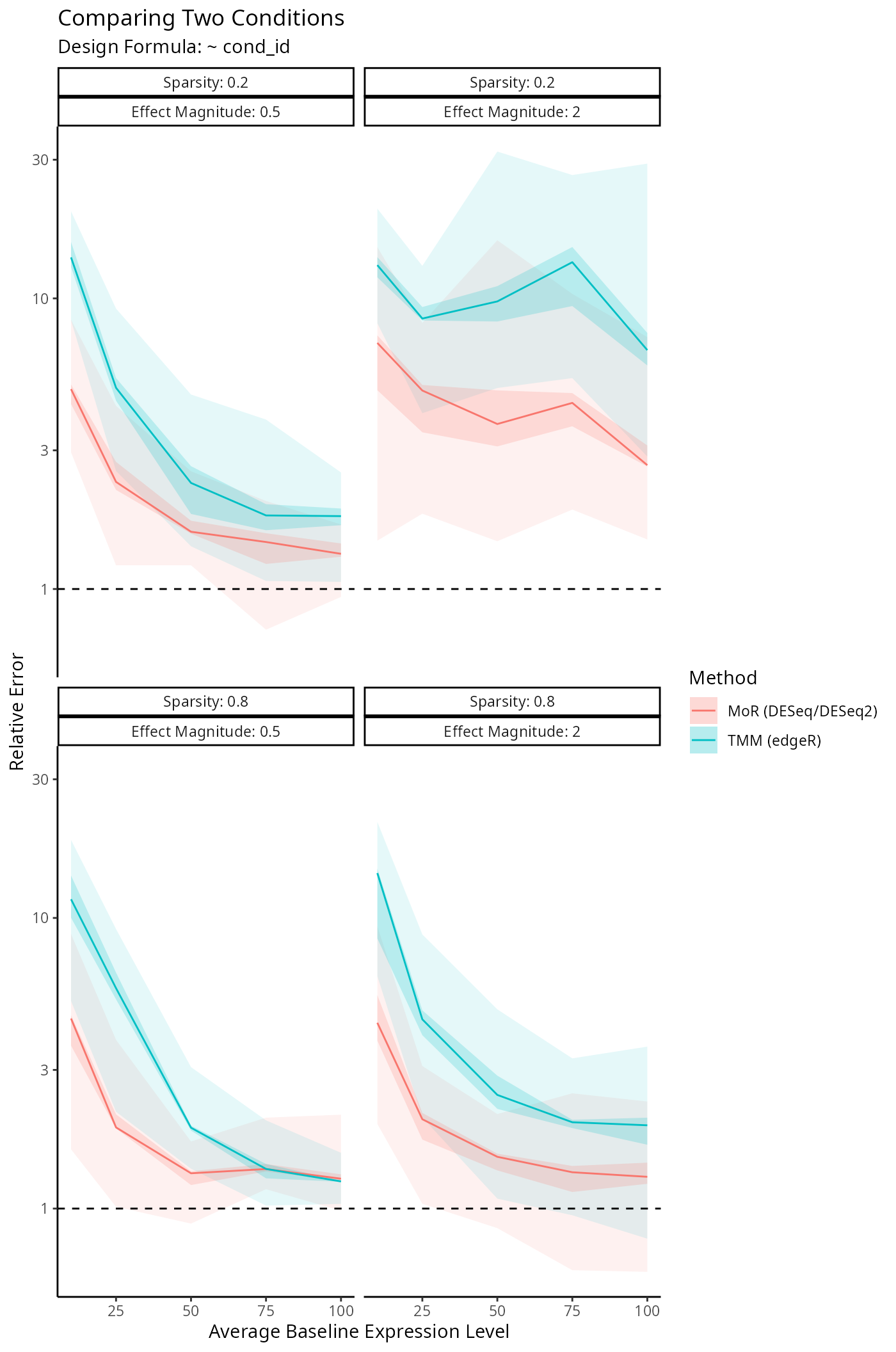
Benchmarking Size Factor Estimation
We’re interested in how well DESeq2, edgeR
and disize estimate the true size factors underlying a
given dataset. The following simulation framework specifies:
- A fixed experimental design.
- The amount of genes measured in the experiment.
- The fraction of genes who are not affected by a given measured covariate.
- The allowed magnitude of the covariate effect (conditional on the gene being affected).
For all experimental designs we construct various scenarios by varying the above parameters and then simulate a dataset corresponding to a given scenario:
# Simulate a single dataset given its settings
simulate_dataset <- function(
    design_formula,
    metadata,
    n_genes,
    sparsity,
    mgt,
    avg) {
    # Simulate inverse overdispersion factors
    iodisps <- rlnorm(n_genes, log(10), 0.5)

    # Split design formula
    design <- split_formula(design_formula)

    # Construct model matrices...

    # Simulate size factors
    size_factors <- runif(length(levels(metadata$batch_id)), 0.1, 1.0) |>
        setNames(levels(metadata$batch_id))
    batch_effect <- size_factors[metadata$batch_id]

    # Simulate counts
    counts <- sapply(1:n_genes, function(g_i) {
        # Simulate fixed-effects
        sparse <- runif(ncol(fe_design)) < sparsity
        fe_coefs <- ifelse(sparse, 0.0, rnorm(ncol(fe_design), 0, mgt))

        # Simulate random-effects
        re_coefs <- lapply(lapply(remm$Ztlist, nrow), function(n_coefs) {
            sparse <- rep(runif(1) < sparsity, n_coefs)

            ifelse(sparse, 0.0, rnorm(n_coefs, sd = mgt))
        }) |>
            unlist()

        # Compute realized magnitude
        log_mu <- as.vector(
            rnorm(1, log(avg)) +
                fe_design %*% fe_coefs +
                re_design %*% re_coefs +
                log(batch_effect)
        )

        # Draw counts from negative binomial
        rnbinom(nrow(metadata), mu = exp(log_mu), size = iodisps[g_i])
    })

    # Cast to integers
    mode(counts) <- "integer"

    list(
        counts = counts,
        metadata = metadata,
        size_factors = log(
            size_factors / sum(size_factors) * length(size_factors)
        )
    )
}

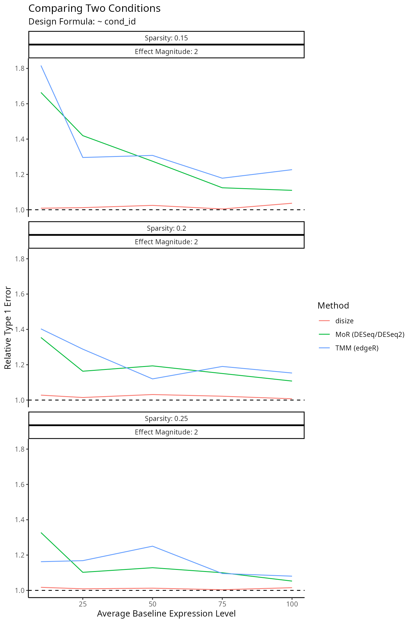
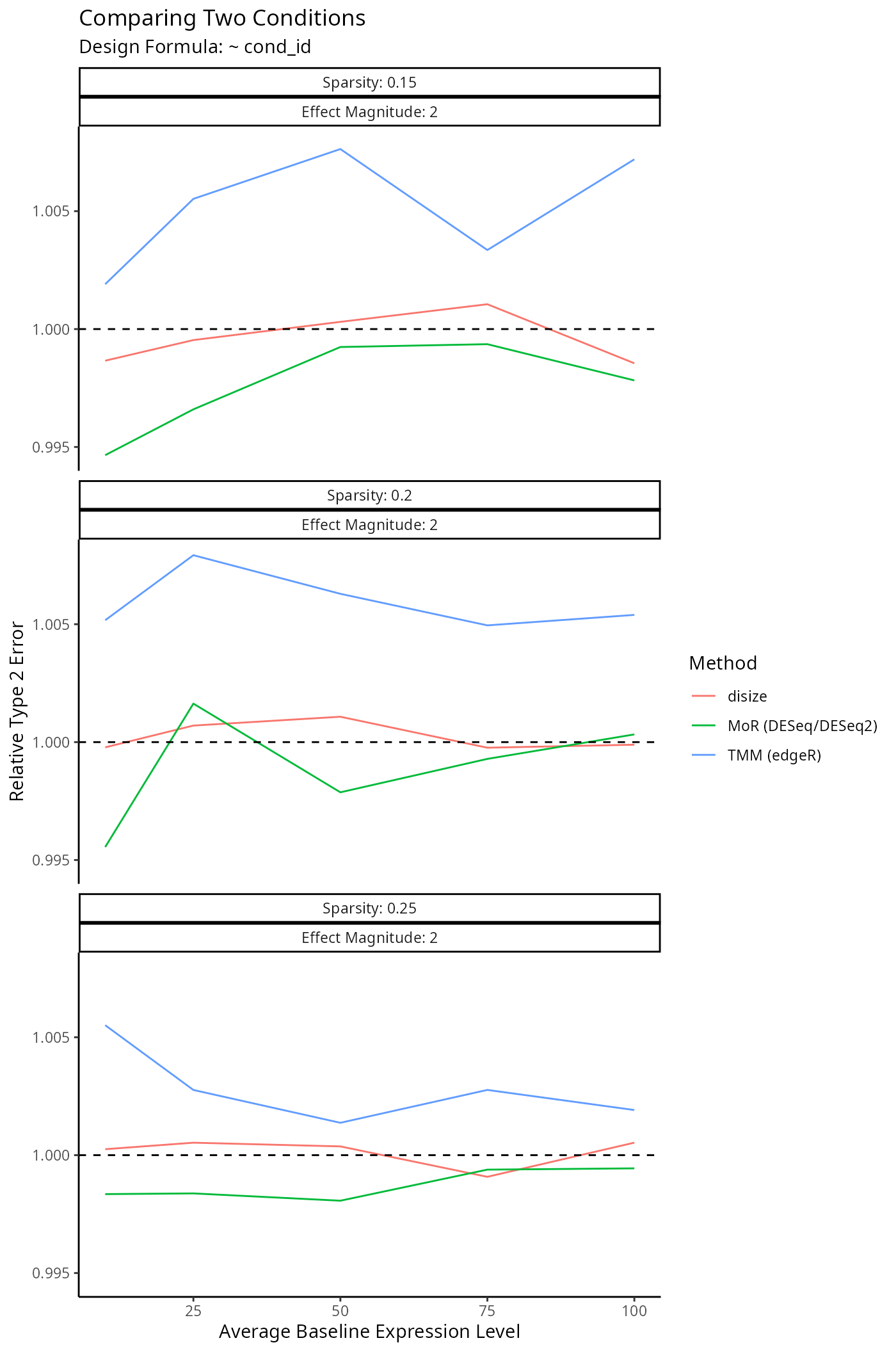
Impact on Downstream Differential Expression Analysis
Normalization is a small component of the transcriptomic workflow. The impact on downstream analyses however is the main outcome of interest, as size factors are only used to account for batch-effects.
To evaluate the impact of each normalization method on a typical downstream analysis, we specify a given experimental design and simulate a dataset similar to the benchmarks above:
# Simulate a single dataset given its settings
simulate_dataset <- function(
    design_formula,
    metadata,
    n_genes,
    sparsity,
    mgt,
    avg) {
    # Simulate inverse overdispersion factors
    iodisps <- rlnorm(n_genes, log(10), 0.5)

    # Simulate size factors
    size_factors <- runif(length(levels(metadata$batch_id)), 0.1, 1.0) |>
        setNames(levels(metadata$batch_id))
    batch_effect <- size_factors[metadata$batch_id]

    # Construct sparsity mask
    mask <- rep(1.0, n_genes)
    mask[1:floor(sparsity * n_genes)] <- 0.0

    # Construct design matrix
    design <- model.matrix(design_formula, metadata)

    # Simulate counts
    counts <- sapply(1:n_genes, function(g_i) {
        # Simulate effects
        effects <- rnorm(ncol(design), sd = mgt)

        # Compute realized magnitude
        log_mu <- as.vector(
            rnorm(1, log(avg)) +
                design %*% effects * mask[g_i] +
                log(batch_effect)
        )

        # Draw counts from negative binomial
        rnbinom(nrow(design), mu = exp(log_mu), size = iodisps[g_i])
    })

    # Cast to integers
    mode(counts) <- "integer"

    list(
        counts = counts,
        metadata = metadata,
        size_factors = log(
            size_factors / sum(size_factors) * length(size_factors)
        ),
        null = mask == 0.0
    )
}
The only difference being we now keep track of which genes are truly null to benchmark the type 1 & type 2 error rates.